Raphaël Errani, CMU

| | | |

nbopy: tools for generating equilibrium N-body models and embedded massless tracers
; ; plots here are copied from .

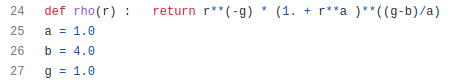
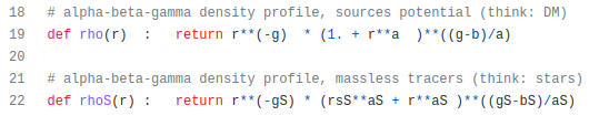
: The code generates equilibrium N-body realisations of spherical, self-gravitating models with isotropic velocity dispersion, following the procedure described in . The desired density profile needs to be specified; the example code on github generates a Hernquist profile.

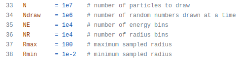
The main parameters to adapt are the number of particles to generate, as well as the resolution of the energy and radius grids used to sample the density profile and the distribution function.

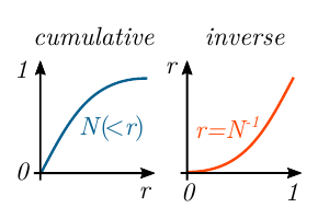
The positions of the N-body particles are drawn using inverse transform sampling from the desired density profile.

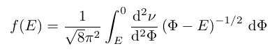
The distribution function is approximated through a numerical evaluation of the Eddington equation.

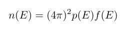
Combined with the density of states

the differential energy distribution is computed.

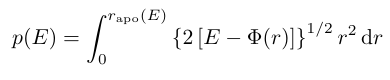
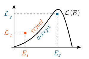
In a final step, for each position r, the likelihood is computed of a particle to have a velocity of v. Isotropic velocities are drawn from this likelihood through rejection sampling.

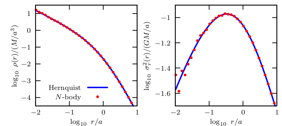
The output is a 6D array of positions and velocities. Below, as an example, density and radial velocity dispersion for a Hernquist sphere generated using the code. The N-body realization shown has N=10⁷ particles generated for radii in the range -3<log₁₀(r/a)<+3. For reference, the analytical Hernquist density- and radial velocity dispersion profiles are plotted in blue.

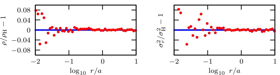
The corresponding residuals are as follows, symmetric around the x-axis, with the effects of discreteness noise visible in the central regions:

The code can be easily adapted to generate other spherical models with isotropic kinematics. Adapting the parameters to α=2, β=5, γ=0, for example, produces a Plummer model as shown below.

Launching the (nbody.py) produces a N=10⁷ particle model of a Hernquist sphere, and saves the particle positions and velocities as a binary numpy file model.npy in 'float16' format (for calculations that use the particle data directly, it is advisable to change the format to 'float64'). Changing the model name in the code to model.dat produces ASCII output.

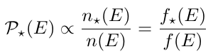
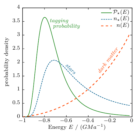
: This is an implementation of the Bullock & Johnston 2005 method for associating stellar weights to N-body models, following the steps described in . The parameters which control the code are near identical to those of nbody.py. In addition to the density profile which sources the potential, the tracer density profile needs to be defined.

Tagging probabilities are computed for spherical, isotropic systems, assuming that stars are massless tracers of the underlying potential. The probabilities are proportional to the ratio of the stellar and dark matter distribution functions at fixed energy.

The probabilities need to be computed only once, and can then be applied to all simulation snapshots. The figure below shows two example differential energy distributions of a dark matter halo and an embedded stellar tracer, as well as the resulting tagging probabilities.

Launching the (first nbody.py, then npaint.py) loads the previously produced N=10⁷ particle model of a Hernquist sphere and computes tagging probabilities for an embedded Plummer model with a scale radius of 20 per cent of the Hernquist scale radius. The probabilities are saved as a numpy file called stars.npy.

: This script generates Gadget2 compatible HDF5 files from N-body models built using nbody.py. It also re-scales the nbody.py model (with M=1, r_s=1) to physical units, as illustrated below:

The code allows to re-define the center of the N-body model, and its systemic velocity:

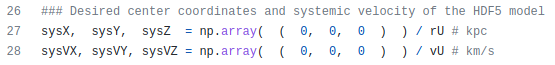
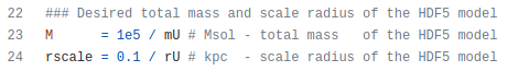
Launching the reads the original model.npy (generated using nbody.py), and saves a Gadget2 compatible HDF5 file to model.hdf5.

tipy: an empirical model for the tidal evolution of NFW subhalos and embedded dwarf galaxies
; papers ,

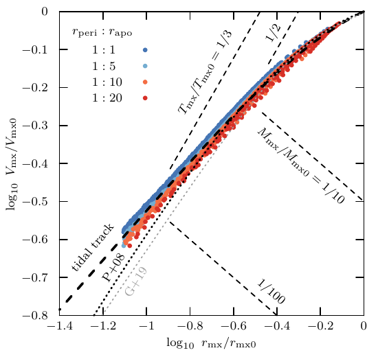
, : This code is an implementation of the empirical tidal evolution model, outlined below.

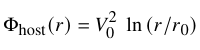
The model parameters are calibrated to the tidal evolution of NFW subhalos orbiting within an isothermal potential.

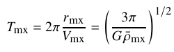
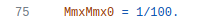
The main parameter determining the subhalo tidal evolution is the initial density contrast of the subhalo with respect to the host at pericentre. The host crossing time at pericentre equals:

The host properties are specified in the code through the pericentre distance r_peri, the ratio of apo-to-pericentre r_apo/r_peri, the orbital period T_orb, and the period of a circular orbit at pericentre, T_peri.

Similarly, the characteristic density of the subhalo is described through the crossing time T_mx at the radius r_mx where its circular velocity curve peaks.

In the code, the initial subhalo structure is defined through the its radius of maximum circular velocity r_mx and the circular velocity V_mx at that radius.

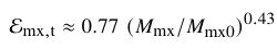
The model empirically describes the full time evolution of the subhalo structure towards the final asymptotic remnant state. For subhalos with an initial crossing time of T_mx0/T_peri>2/3 (the heavy mass loss regime), the subhalo crossing time in the final remnant state is set by the host crossing time at pericentre alone:

The final density profile is that of an exponentially truncated cusp.

Subhalos evolve along well-defined tidal tracks, as introduced in Peñarrubia et al. 2008: the subhalo structure depends only on how much of the initial mass was lost through tides, but not on the orbit. The tidal tracks used in this implementation are as fitted in , with α=0.4 and β=0.65.

The tracks are shown as a black dashed curve in the plot below, with N-body models evolved on different orbits shown in different colours.

For ease of use, the (tipy.py) can be run without any modification to produce an example subhalo tidal evolution as a function of time.

, : This bit of code computes the tidally evolved energy distribution of stellar tracers embedded in a dark matter subhalo using the procedure introduced in . The evolved energy distribution, together with the evolved potential, can later be used to derive the evolved stellar density profile and velocity dispersion.

The model describes tidal evolution through a truncation in energy in the initial conditions. In the following, energies per unit mass

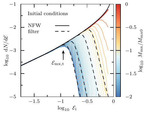
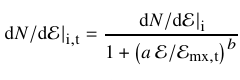
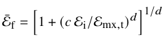
are measured relative to the initial subhalo ground state.

In these units, ε=0 corresponds to the most-bound state, and ε=1 to the boundary between bound and unbound (the plots below show the logarithm of ε). As tidal stripping progresses, the energy truncation (black dashed curves) moves towards more-bound energies, right-to-left in the plot below.

The shape of the tidal energy truncation may be approximated through the following function:

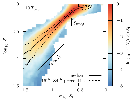
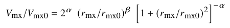
with a=0.85 and b=12. The peak ε_mx,t of the truncated Energy distribution correlates with the final bound mass fraction M_mx/M_mx0 after relaxation.

The relaxation process is modelled empirically through the initial-to-final energy mapping measured from N-body models. The plot below shows such an energy map for a subhalo that has been evolved for 10 orbital periods on an eccentric orbit. The mapping preserves the order in energy in the initial conditions: on average, the most-bound particles in the initial conditions will also be the most-bound particles in the relaxed remnant.

The mapping is parametrised through the following fit:

Stars embedded in the dark matter subhalo are subject to the same tidal truncation as the dark matter. Applying the same formalism to the stellar energy distribution allows to model the evolution of the stellar component. Appendix G in lists the different steps involved in computing the final energy distribution. The (dNde.py) parametrises the initial stellar energy distribution through the function

In the above equation, the parameter α determines how the number of stars drops towards lower energies, while the parameter β determines how sharply stars are truncated beyond the scale energy ε_s. For α=β, the scale energy coincides with the energy where dN/dε peaks. The figure below compares stellar profiles of this parametric energy distribution with Plummer- and exponential models with a projected half-light radius of R_h = r_mx/4.

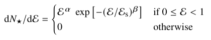
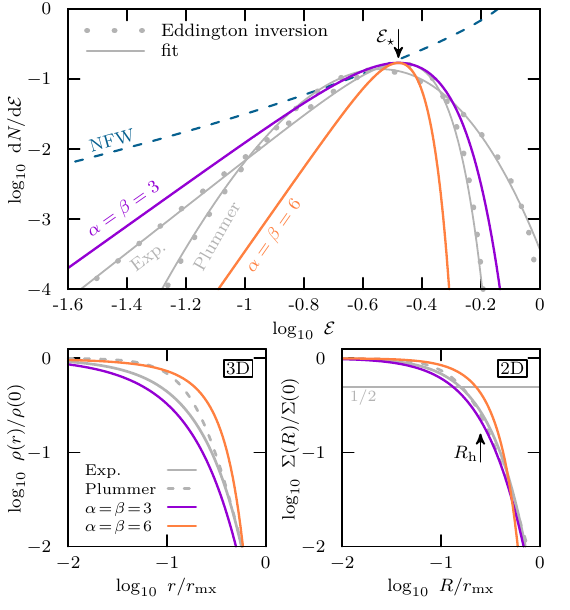
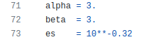
The (dNde.py), as an example, is set up to model the evolution of a stellar tracer with initial α=β=3, and a peak of the initial stellar energy distribution at log₁₀(ε_s)=−0.32.

The surrounding NFW subhalo has been stripped to a remnant mass M_mx of one per cent of its initial mass M_mx0.

The evolved stellar energy distribution is saved as an ASCII table in the file final_dNde.dat.

: This bit of code can be used to generate surface density maps of sparse simulation data. It takes 2D coordinates of N-body particles, maps them on a grid, and subsequently expands each non-empty grid cell until it contains a set minimum number of particles. Each pixel of the output grid is assigned the average surface density of all expanded grid cells that overlap on it. The figure below illustrates how the non-empty grid cells are expanded until each of them contains at least two particles. 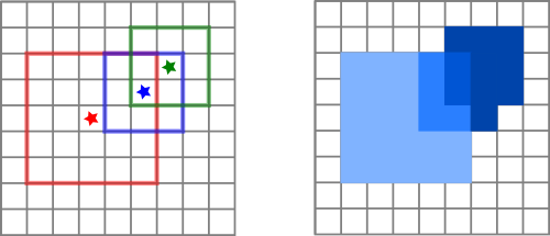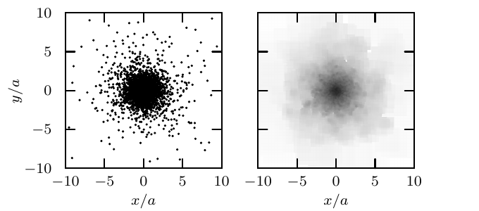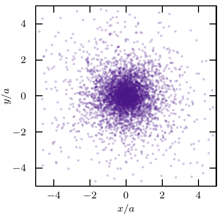The resolution in different regions of the output grid can be intuitively read off from the expanded grid cell size.

The runs a minimum working example upon launch: The ASCII file Plummer.dat is read, which contains x,y coordinates of an N-body Plummer model (shown below in the left-hand panel). The output is written to the ASCII file map.dat, which contains x,y pixel coordinates, as well as the average surface brightness at each pixel (plotted below in the right-hand panel).